AWS XRAY tracing. Part 2: Advanced. Querying & Grouping.

Posted Mar 21, 2023 Updated Feb 25, 2024

By Roman Tsypuk 5 min read

Abstract

Welcome to the next part of our AWS X-Ray series. We’ll explore the flow of trace detection and how to specify different parameters like time ranges. Additionally, we’ll take a deep dive into the DSL of advanced querying. We’ll also examine what is sampling, how it works and how X-Ray groups can assist with operational efforts.

Link to AWS XRAY tracing. Part 1: Foundational

Link to AWS XRAY tracing. Part 3: Sampling & Billing

Accessing traces from Service Map

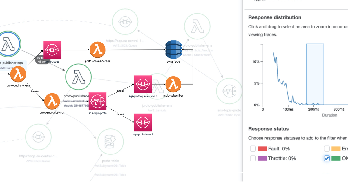
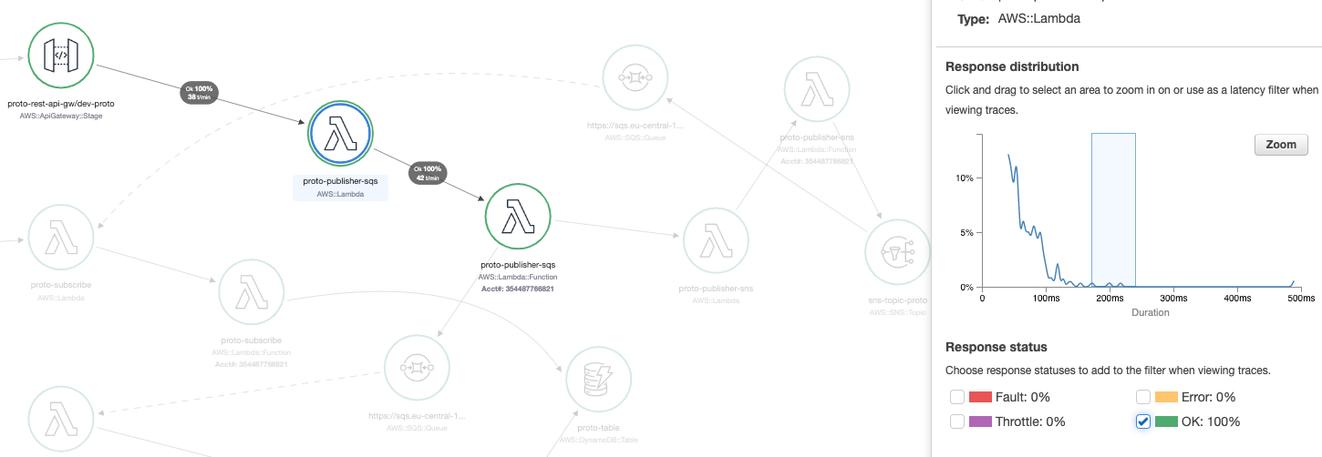
To begin the process, select a dedicated service or edge between services, set a response time range, and choose the desired statuses from the service map:

Once the parameters are specified, the traces will be displayed along with key information such as the trace ID, age, method, response code, response time, client IP, annotation count, and URL: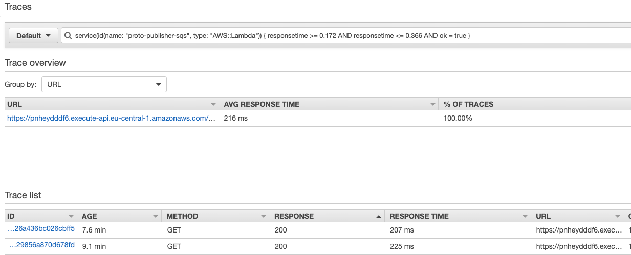

Pay attention to the top section - X-Ray has generated a filter expression to retrieve traces based on your previous selections. To effectively identify issues and bottlenecks, it’s important to be familiar with this DSL. We’ll explore its details later in this post.

service(id(name: "proto-publisher-sqs", type: "AWS::Lambda")) { responsetime >= 0.172 AND responsetime <= 0.366 AND ok = true }

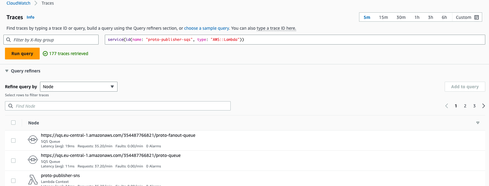
Alternative way is to access traces through CloudWatch xray console that has almost same configurations:

In addition, the middle chart provides useful metrics by representing the distribution of requests in percentiles:

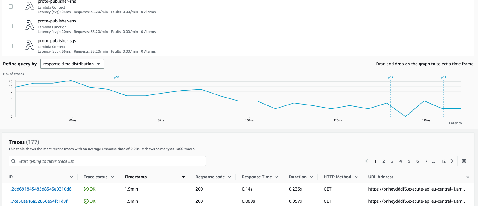
Percentile is a score below which a given percentage of scores in its frequency distribution falls (“exclusive” definition) or a score at or below which a given percentage falls (“inclusive” definition). Percentiles are expressed in the same unit of measurement as the input scores, not in percent The 25th percentile is also known as the first quartile (Q1), the 50th percentile as the median or second quartile (Q2), and the 75th percentile as the third quartile (Q3).

This dashboard also allows you to select the percentile range you’re interested in. For instance, if there are anomalies or spikes in performance, you can narrow down the results by selecting traces within that range for further verification. By changing the percentile range, the query will be updated and the trace results will be filtered accordingly:

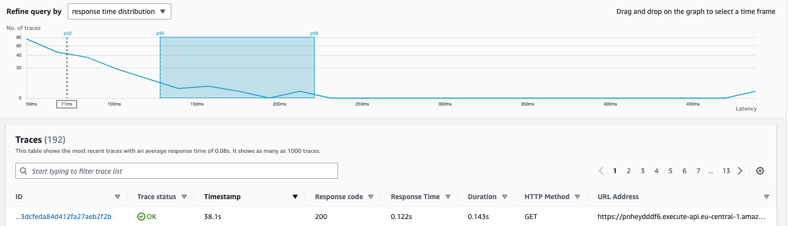
P50 the 50th percentile (median) is the score below contains 50% of the requests in the distribution. So from our chart we observe that 50% requests have latency less than 70ms. P95: 95% requests have latency 132ms or less.

Once we’ve selected the trace ID we’re interested in, we can navigate to the Trace and Segments detail: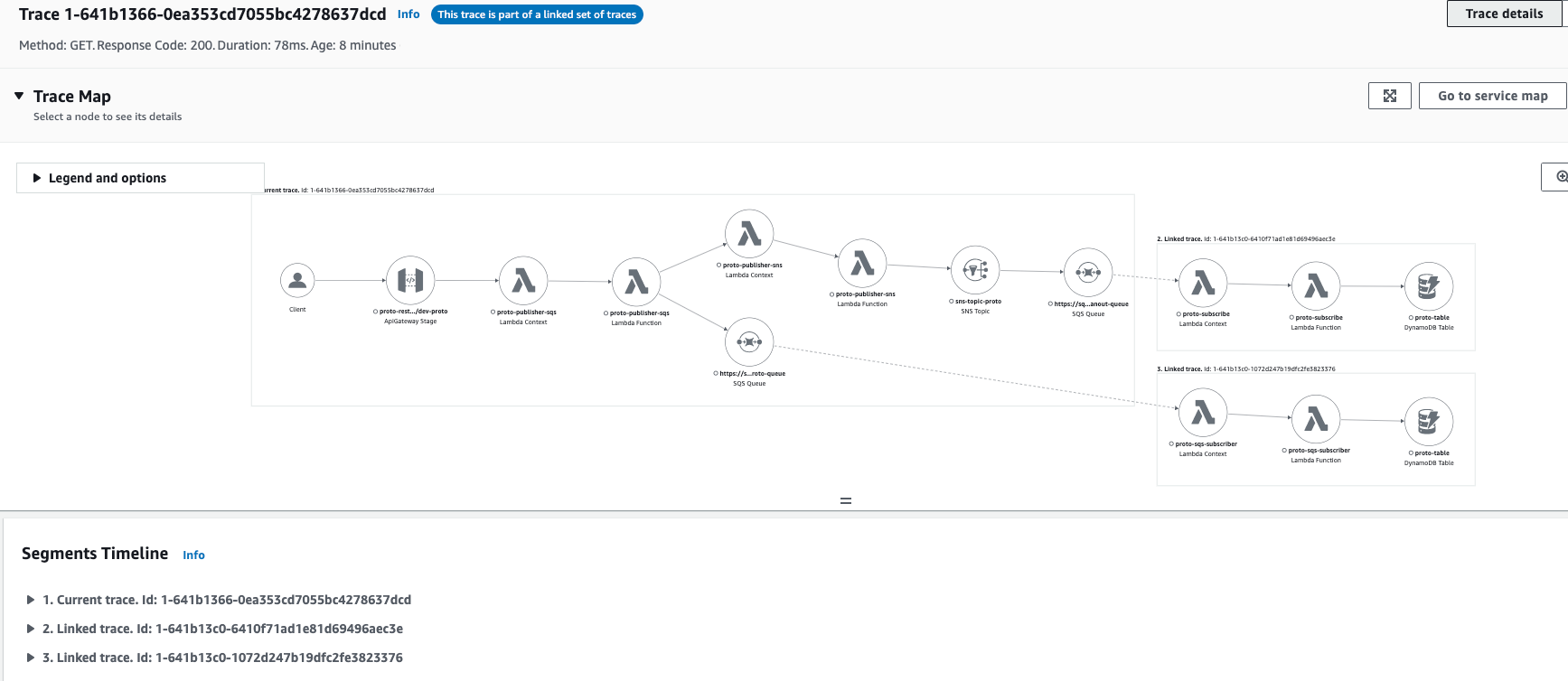

We can observe that this flow is combined from 3 segments. This is due to there are 2 SQS inside the flow that are dividing ecosystem into 3 parts that are producers or consumers. 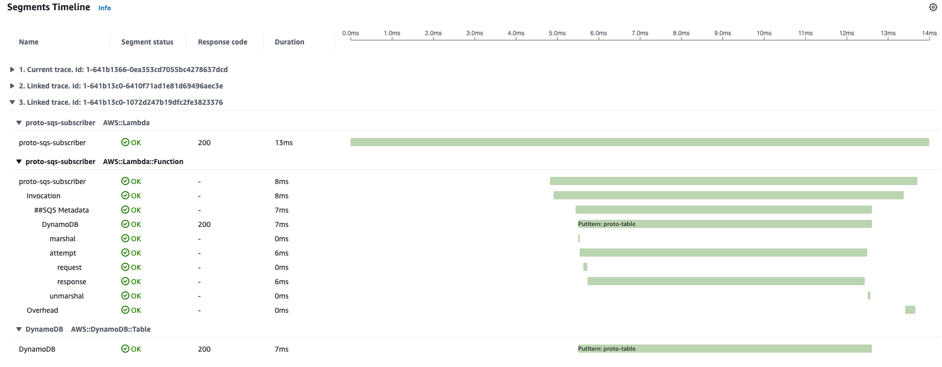We can open and check the details of any linked segment with its traces to check latencies, health and interaction with internal resrouces.

Advanced querying DSL

Now let’s take a look in details of the DSL. There are several operational modes:

Edge level DSL to get connections between AWS services

edge(source, destination) {filter}

Query all traces for flows that have interaction between proto-publisher-sns lambda function and SNS topic:

edge(id(name: "proto-publisher-sns", type: "AWS::Lambda::Function"), "sns-topic-proto")

Same edge connection with additional filtering:

edge(id(name: "proto-publisher-sns", type: "AWS::Lambda::Function"), "sns-topic-proto"){ok = true }

Service level DSL for traces going through AWS service

service(name) {filter}

Query all traces of flows that are going through specified lambda function:

service(id(name: "proto-publisher-sqs", type: "AWS::Lambda"))

Same service query with additional filtering:

service(id(name: "proto-publisher-sqs", type: "AWS::Lambda")) { responsetime >= 0.172 AND responsetime <= 0.366 AND ok = true }

Traces that interact with lambda functions:

service(id(type: "AWS::Lambda"))

Failed lambda functions with errors:

service(id(type: "AWS::Lambda")){fault}

service(id(type: "AWS::Lambda")){error}

ID unique object in AWS environment

In Edge and Service queries id function is used. It allows to narrow the scope to dedicated service based on defined preconditions with pattern: id(name: "service-name", type:"service::type", account.id:"aws-account-id")

After defining the id it can be passed to service or edge DSL:

service(id(type: "AWS::Lambda") to get all lambda functions

service(id(account.id: "xxxxxxx")) - traces that are interacting with entities from other AWS account (if centralized monitoring/tracing account is used).

Annotations and its values also allow querying in DSL

annotation.KEY

Query traces with Subsegments that have annotation MemoryLimitInMB

annotation.MemoryLimitInMB

Same query with values filtering (any memory except 128M)

annotation.MemoryLimitInMB != 128

Subsegments that contain ADMIN annotation

annotation.ADMIN

Subsegments that do not contain ADMIN annotation

!annotation.ADMIN

Lambda functions that have segments with user ‘BOB ‘

service(id(type: "AWS::Lambda")) AND user = 'BOB'

HTTP specific queries including status codes, IP, latencies

http.status != 200

responsetime > 0.2

http.url CONTAINS "/api/proto/"

http.method = GET

http.useragent BEGINSWITH curl

http.clientip = 8.8.8.8

Group queries

group.name = "low_latency_services"

Grouping only services and components that you are interested in (not entire ecosystem)

Using groups on the Service map enables a more focused view of the elements present, displaying only the components that interact with traces following the defined group criteria. This feature is particularly valuable when dealing with complex ecosystems of components, such as those involving data processing, API request and response flows, and asynchronous workers based on queues. With multiple flows and components, the landscape can become overwhelming, making it challenging to observe only the elements currently relevant to your interests. The use of groups helps streamline this process by allowing for a more tailored and efficient analysis of the system.

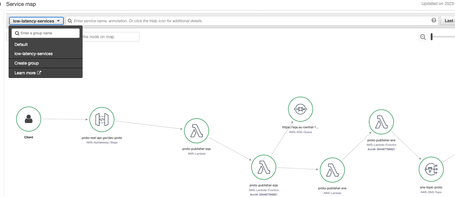
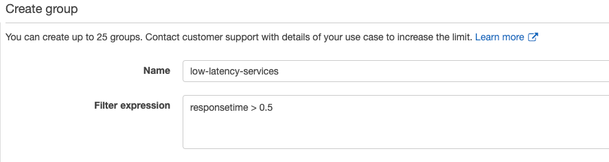
For instance, in the following example, a troubleshooting group named low_latency_services has been created with a filter expression of responsetime > 0.5

Interaction with groups from aws cli

Also, we can perform CRUD operations with xray groups using aws cli:

aws xray create-group
aws xray get-groups
aws xray update-group
aws xray delete-group

  
aws xray get-groups
{
    "Groups": [
        {
            "GroupName": "Default",
            "GroupARN": "arn:aws:xray:eu-central-1:xxxxxxxx:group/Default",
            "InsightsConfiguration": {
                "InsightsEnabled": true,
                "NotificationsEnabled": false
            }
        },
        {
            "GroupName": "low-latency-services",
            "GroupARN": "arn:aws:xray:eu-central-1:xxxxxxxx:group/low-latency-services/UYCODCEBA",
            "FilterExpression": "responsetime > 0.5",
            "InsightsConfiguration": {
                "InsightsEnabled": true,
                "NotificationsEnabled": false
            }
        }
    ]
}

Conclusion

xray is a robust tool that provides a broad range of capabilities, and we have only begun to scratch the surface in this and previous posts. In the next series, we will continue delving deeper.

References (Links)

aws, xray, monitoring

This post is licensed under CC BY 4.0 by the author.